Location, Location, Location
Project Overview
A store chain in Texas has 13 stores throughout the state. This year, the chain would like to expand and open the 14th store. I have been tasked to perform an analysis to recommend the City for the newest store, based on predicted yearly sales.
For this project, I will use a clean dataset to train a linear regression model to predict sales for the prospective new store.
Business Requirements
Here are the criteria’s in choosing the correct City:
The new store should be in a new city. That means there should be no existing stores in the new City.
The total sales for the entire competition in the new City should be less than $500,000.
The new City where you want to build your new store must have over 4,000 people (based upon the 2014 US Census estimate).
The predicted yearly sales must be over $200,000.
The City chosen has the highest predicted sales from the predicted set.
Data Understanding
I have the following information to work with:
The monthly sales data for all the stores for the year 2010.
NAICS data on the most current sales of all competitor stores where total sales are equal to 12 months of sales.
A partially parsed data file that can be used for population numbers.
Demographic data (Households with individuals under 18, Land Area, Population Density, and Total Families) for each City and county in the state of Texas.
Approach
Step 1 - Build a Linear Regression Model: Analyse the dataset and look at the distribution of the data. Histograms are helpful when inspecting continuous and categorical data to determine the nature of the data.
Step 2 - Perform the Analysis: Use a regression model to calculate predicted sales for all the cities and use the criteria given to make a recommendation.
Step 1: Linear Regression
I first plotted each predictor variable against my target variable:
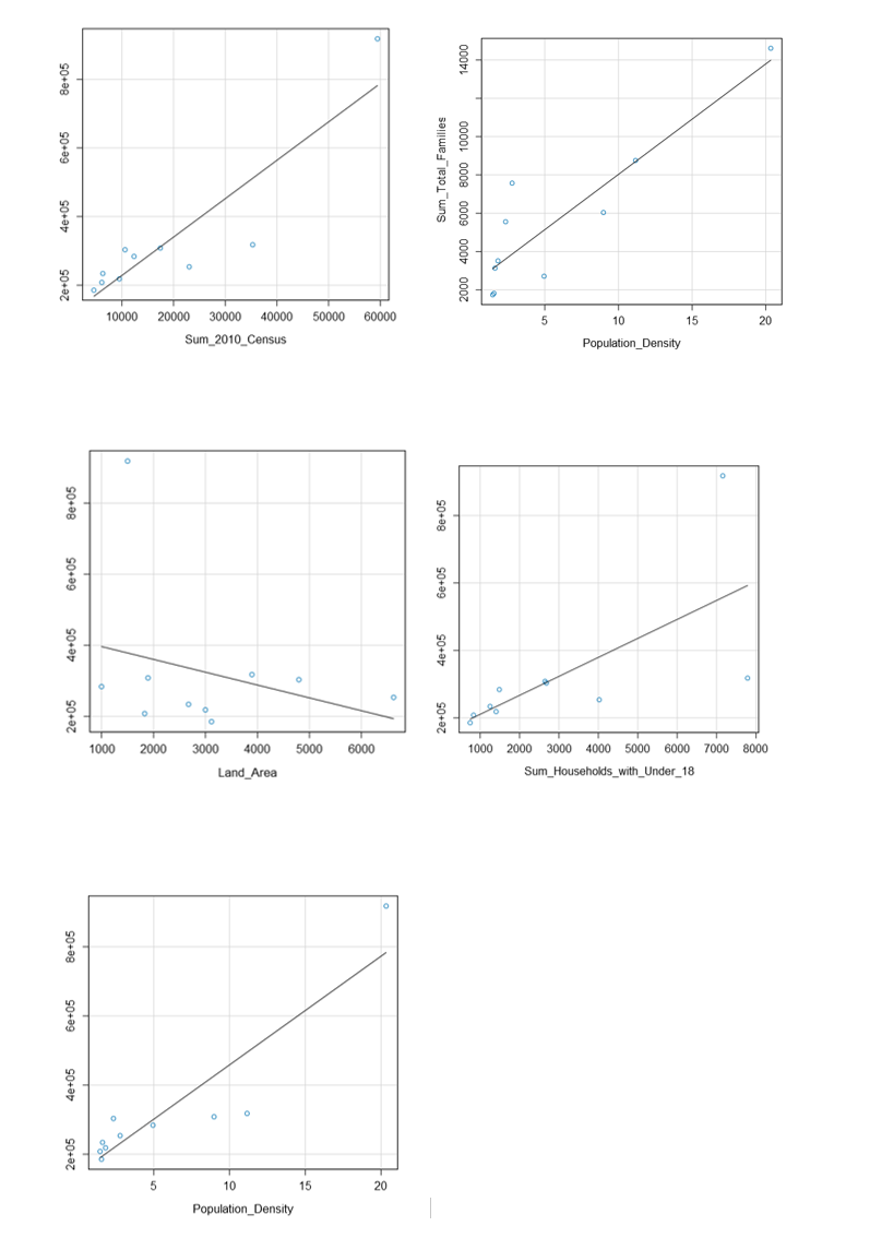
All predictor variables are relevant potential predictor variables because they show a linear relationship between sales. I also checked for correlations between the predictor variables to check for the possibility of multicollinearity.
We see that HHU18, Census, Families, and PDensity (Population Density) have strong correlations with each other. Land area, however, is not as highly correlated. So, I started by using land area as one predictor and then tested the four correlated variables.
I’ve found that using land area and total families as the predictor variables produced the ‘best’ model.

The p-values for land area and total families are both below 0.05, and the Multiple R-squared value is at .91, which is close to 1.
Y = 197,330 – 48.42 * [Land Area] + 49.14 * [Total Families]
Step 2: Analysis
I started with the Web Scraped Data from the Texas Wikipedia page. I then used the Text to Columns and Select tools and the Data Cleansing to parse out the City, County, 2010 Census, and 2014 Estimate to remove all extra punctuation.
I used the Auto-field tool to combine all the numbers labelled as String fields for the demographic data.
Before each join, I summarised the amounts by City to ensure that there were no duplicate city names.
For the Sales file, I transposed the data to get City, Month, and Amount and then summarised by City to get the total amount for each City.
From there, I created the data set used to train the regression model.
Once the model was created, I applied the model to the cities that were not already in the Sales file by taking the left output from the join on the sales file.
I took the competitor data with an auto field tool. I joined it with a formula off of the left join to create a 0 in the Competitor Amount so I could union the cities that have no competitor back into the overall dataset. I didn’t want to exclude cities where no competitors are present as this is a core business requirement.
I then applied the filters laid out in the project plan to develop my list of possible cities and sorted on the expected revenue to bring the best choice to the top.
I recommend the City of Houston with a predicted sales of $305,014.